Tick Symbol in Excel: 12 Awesome Ways to Insert Tick and Cross Symbols

A tick symbol in Excel is very useful if you have a task list, to-do list or a checklist and you want to tick off a task or activity once it has been completed. A tick symbol or also commonly known as a tick mark, can also be used to indicate whether something is correct or has been verified. This very comprehensive tutorial will show you 12 awesome ways on how to insert a tick symbol in Excel. First, before we begin, I will discuss what the difference is between a tick symbol and a checkbox as the two are often confused with each other in Excel. Even though the two may look the same, they are not.

The Tick Symbol vs the Checkbox

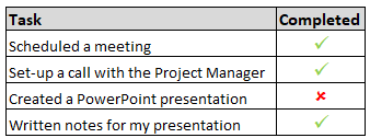
A tick symbol, or tick mark can be inserted in the cell itself. Think of it as a text that you can insert in the cell. Just like with any other text, you can increase or decrease the font size, change its colour, copy it to other cells or delete it by deleting the rows. A cross symbol is often used along with the tick mark to indicate when the task has not been completed.

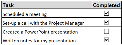
A checkbox is a control that allows you to select or deselect options. It can be inserted from the Developer tab in the Excel ribbon and sits above the worksheet.

What is the Difference between a Tick Symbol and a Checkbox?

There are four main differences between the tick symbol and a checkbox.

1. Firstly, the tick symbol is contained within the cell and the checkbox sits above the worksheet.

2. Secondly, when you delete a row which contains a tick symbol, it will get deleted. With the checkbox, if you delete the row that contains the checkbox, it will not get deleted.

3. Thirdly, you cannot move the tick symbol freely around the worksheet as it is contained in the cell. You would have to cut the cell where the tick symbol is contained and paste it to another cell. With the checkbox, you can freely move it around the worksheet with your mouse as it sits above the worksheet.

4. Lastly, you can easily format a tick symbol. I will show you how to format tick symbols using the formatting buttons in the Excel ribbon and by using conditional formatting later in the post. With the checkbox, you cannot format it.

I will now show you 12 great ways on how to insert tick symbols in Excel. This post will also show you how to insert cross symbols in Excel too.

Copy and Paste a Tick Symbol in a Cell

Copying and pasting is the simplest and easiest method to insert a tick symbol in Excel. One of my favourite sites to get a list of symbols to copy is Made in Text. This website contains a wide variety of symbols in different categories which you can just copy and paste in Excel.

Alternatively, you can just copy the tick mark below by highlighting it with your mouse and pressing Ctrl+C. Then go to Excel and select the cell where you want to paste the tick symbol and then press Ctrl+V to paste it in the cell.

✔

How to Enter a Tick Mark using the Symbol Dialog Box

Excel contains a list of symbols you can insert into your worksheet. You can insert a tick mark using the Symbol command from the Excel ribbon. Below are the steps to do this.

1. Select the cell in the worksheet where you would like to insert the tick mark.

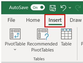
2. Go to the Insert tab in the ribbon.

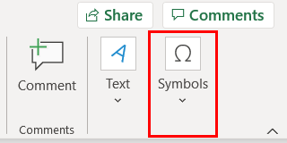
3. Select the Symbols button in the Symbols group.

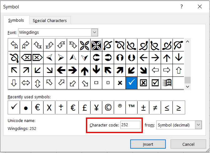
4. The Symbol dialog box will appear. In the Font drop-down box select the Wingdings font.

5. Scroll down right to the bottom using the scroll bar on the right. You will see a couple of tick marks and cross symbols. Select the one that you like and then press the Insert button.

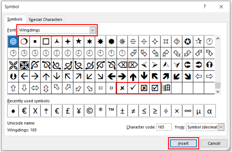
6. The selected symbol will appear in the worksheet. Next, click the Close button to exit the Symbol dialog box.

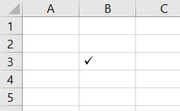
This will insert one tick symbol in the selected cell. To insert further tick symbols, you can repeat the above steps but a much quicker way is to copy the already inserted tick symbol and paste it to the other cells where you want the tick symbols to be.

How to Insert a Tick Symbol using Keyboard Shortcuts

If you like using keyboard shortcuts, and lets be honest, who doesn’t, then you can use them to insert tick marks in Excel. One thing to note is that you must use the Wingdings font in order for this method to work. Below are the step by step instructions to insert a tick symbol in Excel.

1. Select the cell where you want to insert the tick mark.

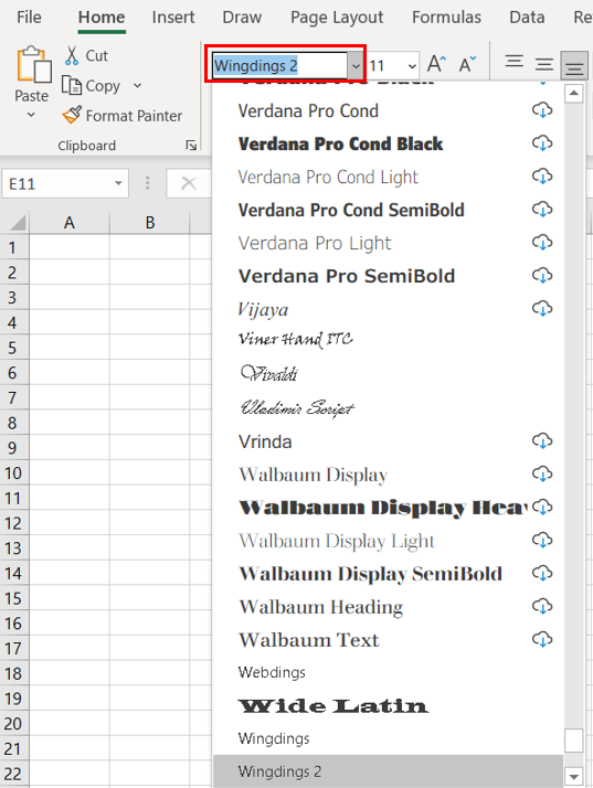
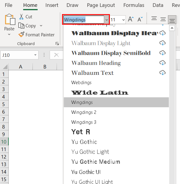
2. Change the font to Wingdings 2 by going to the Home tab in the ribbon and under the Font group click the drop-down arrow to the right of the Font field and select Wingdings 2.

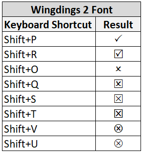
3. Enter one of the keyboard shortcuts from the table below depending on which symbol you want to use.

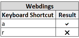
Instead of the Wingdings 2 font, you can also use the Webdings font instead to apply a tick or cross symbol. To do this, follow the above steps but in step 2 choose the Webdings font instead. In step 3, use one of the below shortcuts to insert a tick mark or a cross.

A Quick Note

A point to note is that it is not a good idea to use any other text or numbers in the same cell as the tick or cross mark. This is because the cell is either in the Wingdings 2 or Webdings font. By entering any other text or numbers in the same cell as the tick or cross mark, it will not show correctly in the cell. This method is best suited for when you only want to insert a tick or cross symbol in a cell and nothing else.

Inserting a Tick Mark in Excel by Using it’s Character Code

Following on from the previous method of using keyboard shortcuts, another quick way to insert tick marks is to use its character code. You can do this by using the ALT key on your keyboard while typing in its character code. Like with the previous method, you must change the font to Wingdings to the cells where you want to insert the tick symbols first. Below are the step by step instructions to insert a tick mark by using its character code.

1. Select the cell where you want to insert the tick mark.

2. Change the font to Wingdings by going to the Home tab in the ribbon and under the Font group click the drop-down arrow to the right of the Font field and select Wingdings.

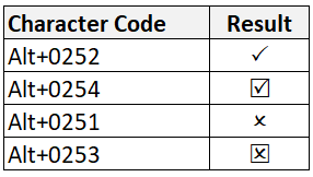
3. Enter one of the character codes from the table below depending on which symbol you want to use.

Some Points to Consider

Some points to note when you enter any of the symbols using their character codes:

• Keep the ALT key pressed while you are entering the numbers.

• Use the numerical keypad rather than the numbers at the top of keyboard, otherwise it will not work.

• As with the keyboard shortcut method mentioned earlier, because the Wingdings font is used, this method is suitable for when you only want to insert a tick or cross symbol in a cell and nothing else.

Tip: if you want to know what the character codes are for other symbols you would like to insert in your worksheet then use the Symbol dialog box which I have already discussed earlier. Select the symbol you like and then at the bottom in the Character code field you will see what the character code is.

Inserting a Tick Mark using the CHAR Function

Another way you can insert a tick mark in Excel is to use the Excel CHAR function. The CHAR function returns a character when you give it a character code. The syntax for the CHAR function is:

=CHAR(code)

For a tick symbol, you simply replace the “code” with the tick symbol’s character code. You must apply the Wingdings font to the formula cells.

Here are the steps to insert a tick symbol in Excel using the CHAR function.

1. Apply the Wingdings font to the cells where you want to insert the tick marks.

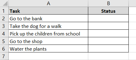
2. Select the cell where you want to insert the formula to return a tick mark. In the example below, I want to insert a tick mark in cell B2.

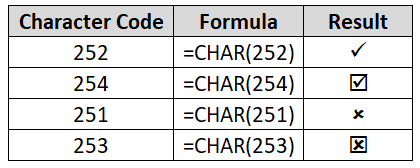
2. In the active cell, type =CHAR(code), replacing “code” with the tick symbol’s character code. The character codes to use for the tick and cross symbols are as follows:

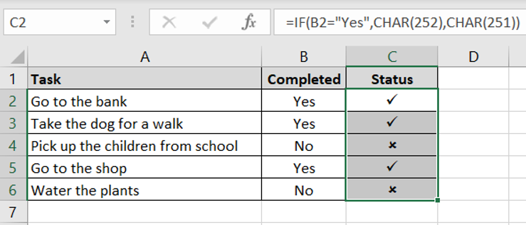
3. The tick symbol has been inserted in the cell. The formula I used in cell B2 is =CHAR(252).

The main benefit of using the CHAR function to insert tick marks is that you can combine it with the IF function to easily insert tick and cross symbols in cells based on a criteria in other cells.

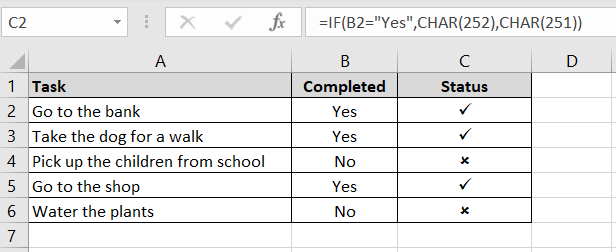
In the above example, I used the below formula in column C to insert a tick if column B says a “Yes” and a cross if it says a “No”.

=IF(B2=”Yes”,CHAR(252),CHAR(251))

Inserting a Tick Symbol in Excel using AutoCorrect

If you want to automate inserting tick symbols in Excel rather than copying and pasting them or using formulas, then a quick way to do this is by using the Excel’s autocorrect feature. This feature in Excel autocorrects words which are spelled incorrectly automatically. Here are the steps to do this.

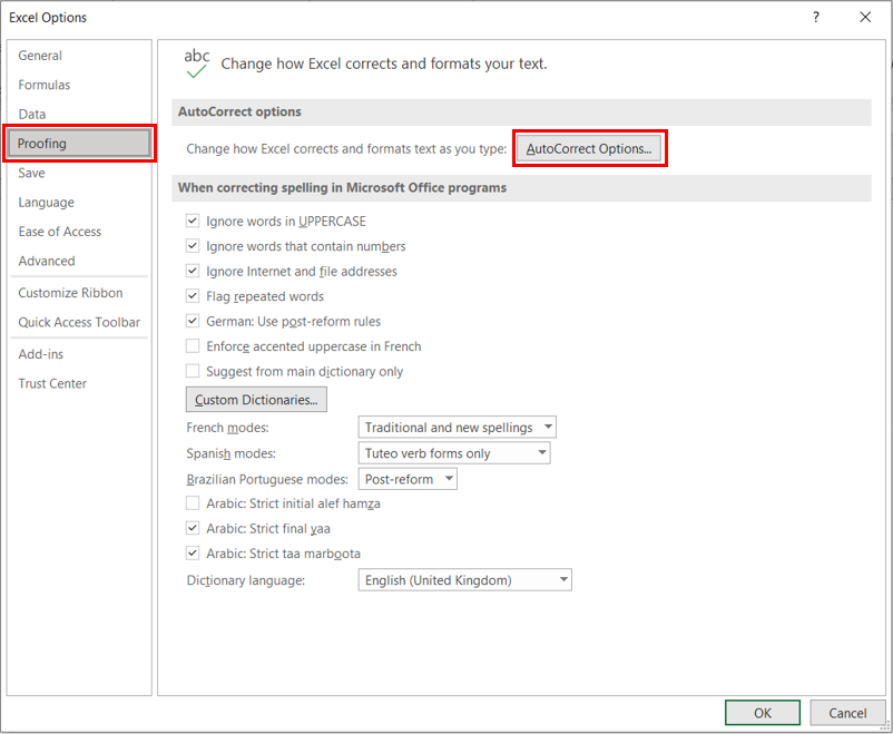
1. Go to the File tab in the ribbon, then click Options.

2. In the Excel Options dialog box, select Proofing and then under AutoCorrect options click on the AutoCorrect Options button.

3. The AutoCorrect dialog box will appear. Under the Replace field, type a word which you will associate with a tick mark. In the example below, I entered TickMark. In the With field insert the tick mark. You can copy the tick mark which is located near the beginning of this post. Next press the OK button.

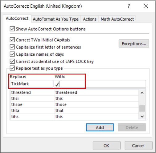
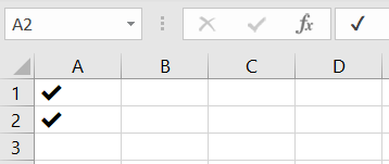
4. Now whenever I type TickMark in a cell, Excel will insert the tick symbol.

Points to Note

• You only have to change the AutoCorrect setting once. Excel will always insert a tick whenever you enter the word for the tick symbol.

• This is case sensitive. If I typed “TICKMARK”, “tickmark”, or “tICKmARK” in a cell, then it will not work. To cover all bases, you can create multiple autocorrects using different cases for the same word.

• When you create an autocorrect to insert a tick mark, it will apply to all other Microsoft Office applications too such as Word and PowerPoint.

• It is highly recommended that you enter a word in the Replace field in the AutoCorrect dialog box that you will not use for anything else.

• If you use any symbols before or after the word, it will not get converted to a tick mark. For example, TickMark$ will convert to ✔$.

How to Insert a Tick Symbol as an Image

If you want the tick marks to stand out more and contain colour then you can use online pictures. To do this, follow these steps.

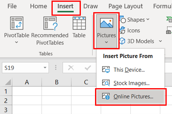
1. From the Excel ribbon, go to the Insert tab. Under the Illustrations group click the Pictures button. From the next menu, select Online Pictures.

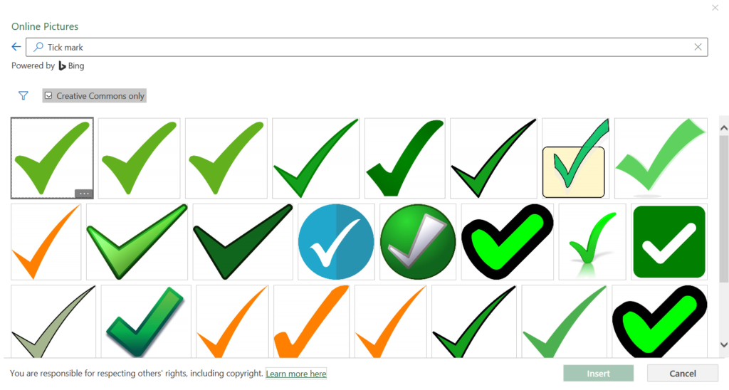
2. The Online Pictures dialog box will appear. In the search bar, type Tick mark and press the Enter key on your keyboard. A variety of tick marks will appear.

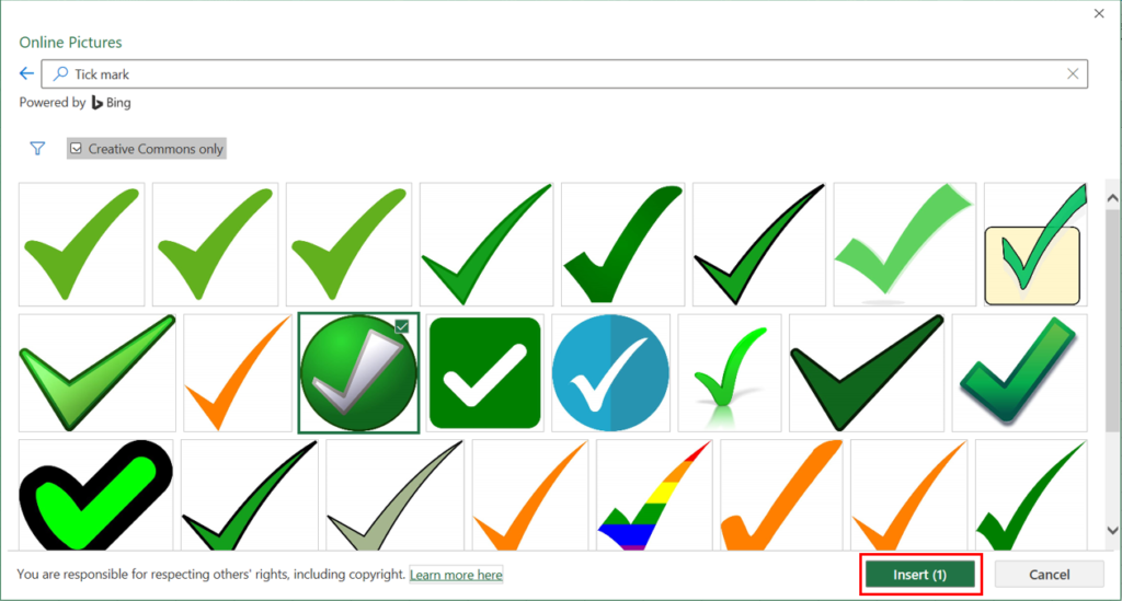
3. Select the tick mark you like and then press the Insert button.

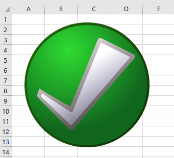
4. The tick mark will be inserted in the worksheet. You can resize it by clicking on the image and using the size handles to make it bigger or smaller. As the image sits above the worksheet, you can move it around anywhere in your worksheet.

How to use Conditional Formatting to Insert Tick Symbols

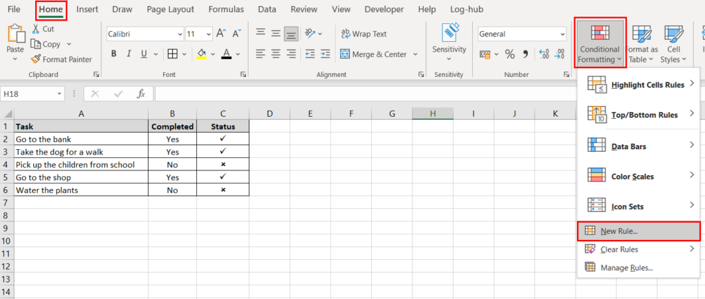
Another great way to insert a tick symbol in Excel is by using Excel’s conditional formatting feature. Excel will insert a tick mark or a cross symbol based on the value in a cell. Here are the steps to do this.

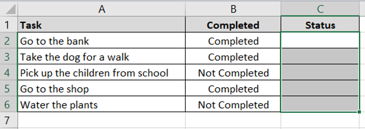
1. Select the cells where you want to insert the tick or cross symbols. In this example, I want to insert them in the range C2:C6 so I select this range.

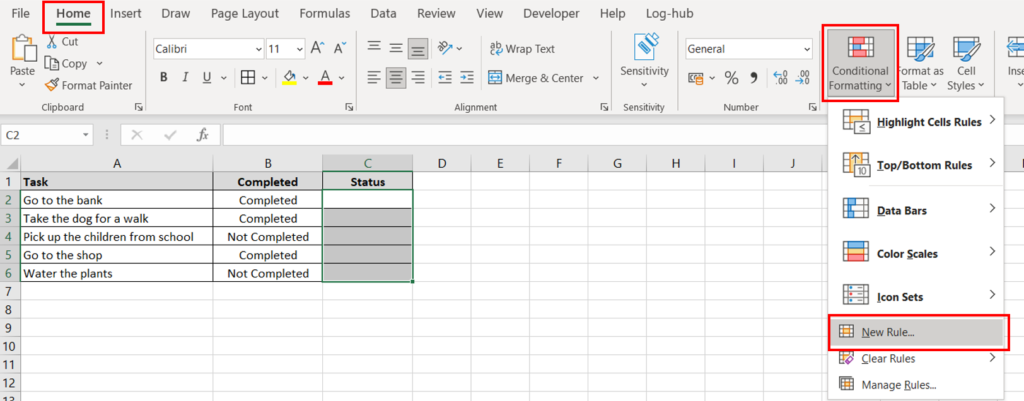
2. In the Excel ribbon, go to the Home tab and then under the Styles group click the Conditional Formatting button. From the menu select New Rule.

3. The New Formatting Rule dialog box will appear. Select the following settings:

• In the Format Style field select Icon Sets from the drop-down list.
• In the Icon Style field select the one with the cross, exclamation mark and tick symbols.
• Check the checkbox where it says Show Icon Only.
• Enter the values under Value. Enter “1” for when you want to show a green tick mark and “0” where you want to show a red cross.
• Under Type, select Number from the drop-down list.
• Under Icon, change the amber exclamation mark to a red cross by clicking the drop-down button next to the icon and then select the red cross from the list.

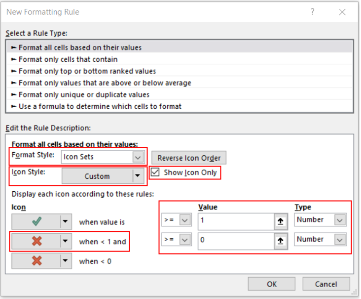
4. Press the OK button to confirm the settings.

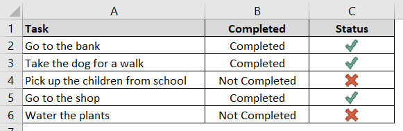
5. Now when I enter a “1” or a “0” in column C, Excel will enter a green tick or a red cross.

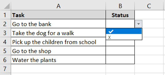
Inserting a Tick Mark using a Drop-Down List

Another method of inserting a tick mark in Excel is by creating a drop-down list which contains the tick mark. You can then use this drop-down list to insert the tick mark into your worksheet. To do this follow these steps.

1. First, copy a tick mark. You can copy the tick mark near the beginning of this post.

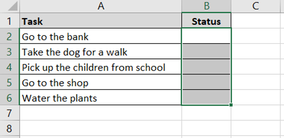
2. Select the cells where you want to insert tick marks. In this example, I want to insert tick marks in the range B2:B6.

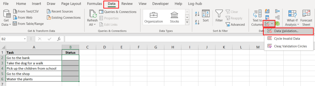
3. From the Excel ribbon, go to the Data tab and then under the Data Tools group, select the Data Validation button. A menu will appear with three options. Select Data Validation.

4. The Data Validation dialog box will appear. Under Allow, select List from the drop-down menu. Under Source, paste the tick mark you copied from step 1.

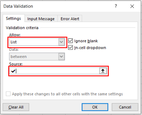
5. Press the OK button.

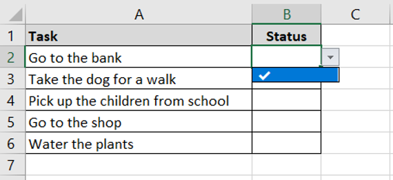
6. Now when you select a cell where you want to insert a tick mark, you can choose the tick mark from the drop-down list.

You can also add a cross symbol to the drop-down list so you can select either a tick or a cross symbol. To do this, simply copy the below cross symbol or copy any of the crosses from the Made in Text website.

☓

Go back to the Data Validation dialog box and then put a comma next to the tick mark. Paste the cross symbol after the comma and then press the OK button.

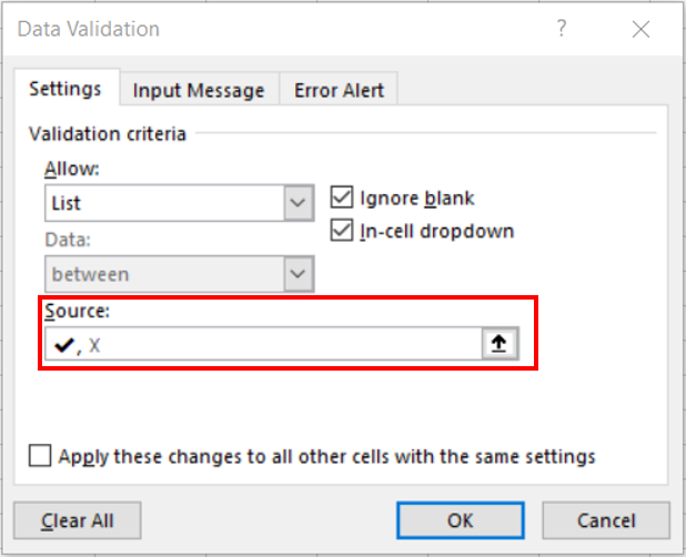
The cross symbol is now included in the drop-down list.

Inserting a Tick Symbol in Excel using a VBA Macro

Macros are a great way to automate your worksheets to save you time and effort. You can create a macro for almost anything. The below code will insert a tick mark in the selected cells.

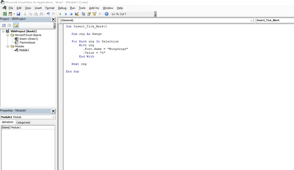
 Sub Insert_Tick_Mark()

   Dim rng As Range

   For Each rng In Selection
       With rng
         .Font.Name = "Wingdings"
         .Value = "ü"
       End With

   Next rng

 End Sub

To insert this VBA code into your worksheet, follow these steps.

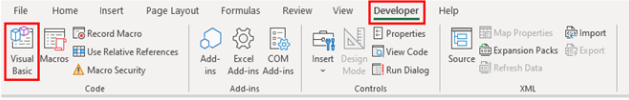
1. Click on the Developer tab in the Excel ribbon. Under the Code group press the Visual Basic Button. Alternatively, press ALT+F11 on your keyboard.

2. The Visual Basic Editor will open. From the menu at the top, click on the Insert tab and then Module from the next menu. This will open up the code window.

3. Copy the VBA code above and paste it in the code window.

4. To run the code, select the cells in your worksheet where you want to insert the tick symbols and then go back into the Visual Basic Editor and click anywhere in the VBA code.

5. Now press the Run Sub/Userform button which looks like a green triangle. Alternatively, you can press the F5 key.

6. The macro has inserted tick marks in the selected cells.

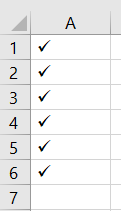
This code works by looping through each selected cell and changes the cell to the Wingdings font and enters the value ü. The Wingdings font will make the ü value into a tick symbol.

Inserting a Tick Symbol using the Double Click Method in VBA

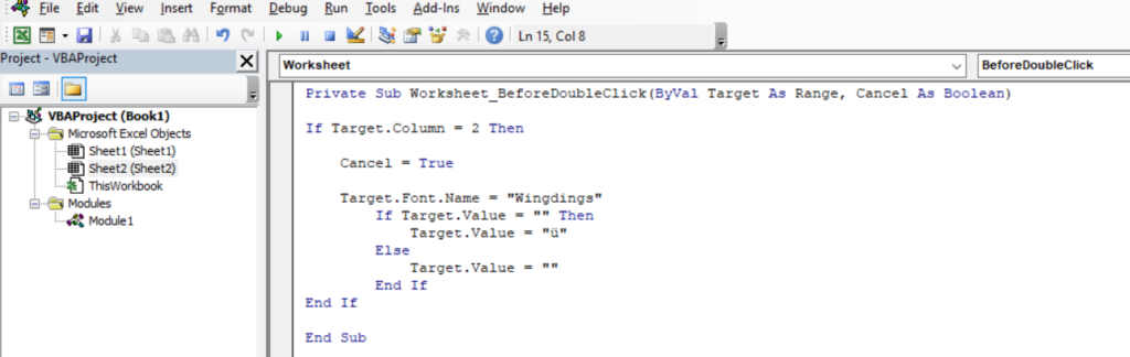
Following on from the previous method of using a VBA macro, you can also use the below VBA code to insert tick marks. This macro inserts a tick mark whenever you double click a cell in column B. It also removes a tick mark by double clicking the cell which contains the tick mark.

Private Sub Worksheet_BeforeDoubleClick(ByVal Target As Range, Cancel As Boolean)

If Target.Column = 2 Then

    Cancel = True

    Target.Font.Name = "Wingdings"
        If Target.Value = "" Then
            Target.Value = "ü"
        Else
            Target.Value = ""
        End If
End If

End Sub

You have to insert the above code in the worksheet where you want to insert the tick marks. To do this follow these steps.

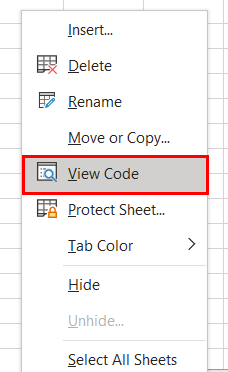
1. Right-click the worksheet tab name and click on View Code.

2. Copy the above code and paste it in the code window.

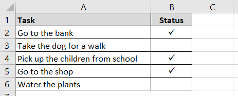
3. Now go back to the worksheet and double click any cell in column B to insert the tick mark.

This code uses VBA’s double-click event. It first checks if the cell you have double-clicked is in column 2, i.e. column B or not. If the cell you have double-clicked is in column 2, then it changes the font to Wingdings. It then checks if the cell is blank or not. If it is blank, then it enters the value ü. If there is already a value in the cell, then it makes the cell blank. This means you can add or remove tick marks by simply double-clicking the cell in column B.

The best use case for this method is if you are going down a list of activities and you are checking off each activity that has been completed.

Using the Draw tab from the Excel Ribbon

If you have Office 365, then you may notice that Excel has a new tab called Draw.

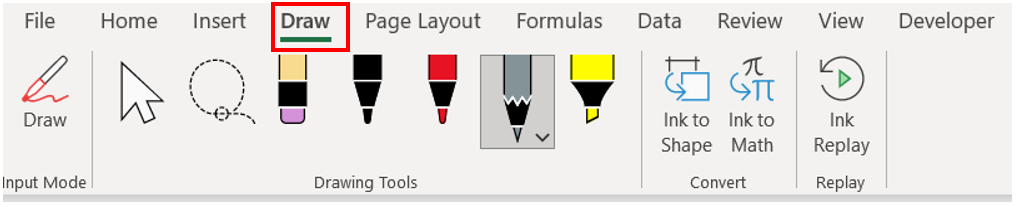
This tab allows you to draw directly into your worksheet. There are various marker pens you can choose from to draw a tick mark. Excel will insert this as an image which will sit on top of the worksheet. You can then make it bigger or smaller and move it around the worksheet. If you are not happy with the tick mark you can simply use the eraser to delete it and then try again.

The best thing to do is to play around with the pens and the various other features in this tab as it allows you to be very creative and you will be able to draw some cool things.

Tick Symbols Tips and Tricks

You have learnt some great methods on how to insert tick marks and cross symbols in your worksheets. This next section will give you some helpful tips and tricks which you can use such as how to apply formatting and how to count tick and cross symbols.

Formatting a Tick Mark

A tick mark is like any other text character. This means you can increase its size, change its colour, make it bold, italic and underline it. Formatting a tick mark is useful when you want to make it stand out.

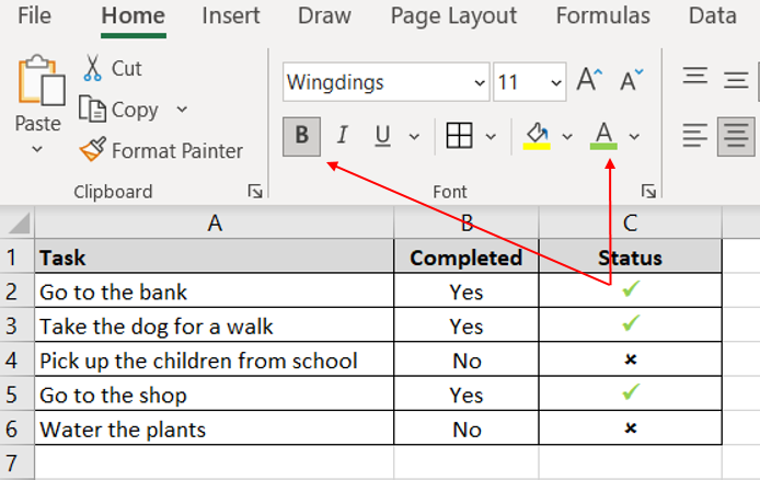
In the screenshot above, I have made the tick symbols green and bold. I first selected the tick marks and then used the Font Color button to change its colour to green and then pressed the Bold button to make it bold.

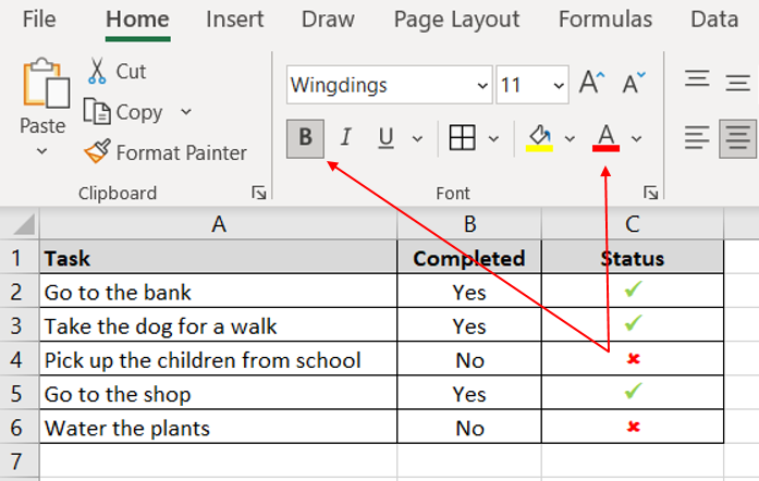
I have then made the cross symbols red and made it bold. Again, I selected the cells which contained the crosses and then pressed the Font Color button to change its colour to red and then pressed the Bold button to make it bold.

Using Conditional Formatting to Format a Tick Mark

Applying formatting to tick marks using the previous method is useful if there is only a few to format. It can take a while if there are many tick or cross symbols to format. A better solution is to use conditional formatting. Another reason why this method is better than the previous method is that you do not need to re-apply the formatting if you have deleted a tick mark. Below are the steps to format tick marks using conditional formatting.

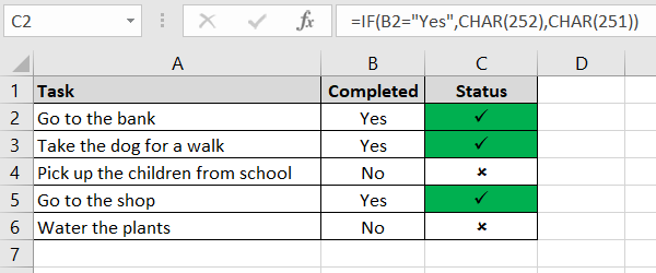
1. Select the cells where you want to apply the conditional formatting to the tick marks. In the example below, I have selected the range C2:C6. I have used the CHAR function to insert the tick and cross symbols in column C.

2. In the Excel ribbon, select the Home tab and under the Styles group press the Conditional Formatting button. From the next menu, select New Rule.

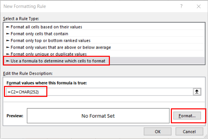
3. The New Formatting Rule dialog box will appear. Select the Use a formula to determine which cells to format and under Format values where this formula is true enter the formula =C2=CHAR(252) and then click the Format button.

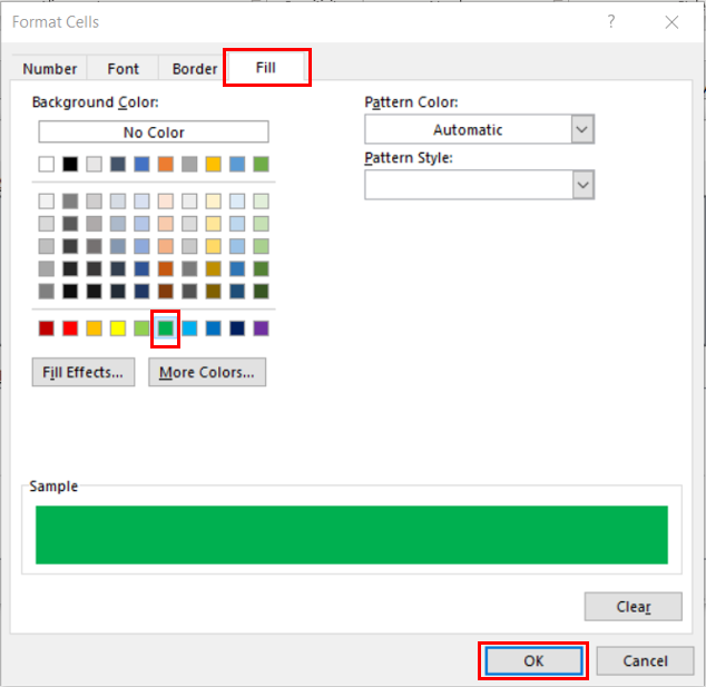
4. The Format Cells dialog box will appear. Go to the Fill tab and select the green colour. Finally, press the OK button.

5. This will take you back to the New Formatting Rule dialog box. Press the OK button and the cells with the tick marks have turned green.

You can format the cells however you wish from the Format Cells dialog box. For example, you can change the font colour of the tick mark and make it bold from the Font tab.

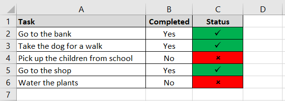
To format the cells with the cross symbols, you follow the same steps as shown above but this time enter the formula =C2=CHAR(251) under Format values where this formula is true in the New Formatting Rule dialog box in step 3.

How to Count the Number of Tick Marks in Excel

If you want to count the number of tick marks and cross symbols you can use the COUNTIF function together with the CHAR function. The CHAR function has already been explained earlier in this post. The COUNTIF function simply counts the number of cells from a given criteria. The syntax for the COUNTIF function is:

=COUNTIF (range, criteria)

The range argument is the range of cells to count and the criteria argument is the criteria you want to count.

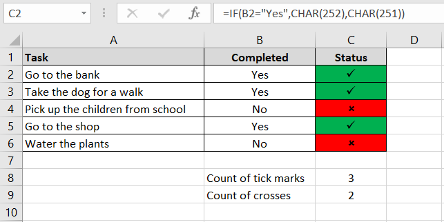
In cell C8, I have inserted a formula to count the number of tick marks in the range C2:C6. The formula is: =COUNTIF($C$2:$C$6,CHAR(252)). This formula counts the number of times the character code 252 is contained in the range C2:C6.

Similarly, I have entered the formula =COUNTIF($C$2:$C$6,CHAR(251)) to count the number of times the character code 251 is contained in the range C2:C6.

Final Word

I have shown you 12 methods of how to insert a tick symbol in Excel. Tick symbols are great when you have a checklist or a to do list to help you keep track of your daily, weekly and monthly activities. You can use any of the methods described above, however choose the one you find the most suitable for your needs. Let me know which is your favourite method in the comments section below. If you know of any more methods to insert a tick mark in Excel then let me know in the comments section below.

Excel in Style: The Top Excel Mugs You Need on Your Desk!

Looking to add a touch of Excel magic to your daily routine? Our Excel mugs are here to enhance your experience. Whether you’re a spreadsheet guru or just appreciate a beautifully designed mug, these are the perfect choice. Elevate your coffee breaks, add some flair to your desk, or find the ideal gift for a fellow Excel enthusiast. Don’t miss out – click to explore our collection and make every sip a spreadsheet sensation!

Learn More Awesome Excel Tips and Tricks

Inserting tick symbols in Excel is just one awesome way of utilising Excel. There are however many other tips and tricks you can use to get the most out of Excel. I have written an Excel book called Excel Bible for Beginners: Microsoft Excel Book Containing the Best Excel Tools, Tips and Shortcuts you Need to Know which will save you hours of time and effort.

Excel Bible for Beginners Book by Harjit Suman

This Excel book will help you work smarter, save time, and become more productive by learning all the best hints, tips and tricks Excel has to offer. This book will show you how to:

• Hide specific text in a worksheet
• Quickly insert multiple rows using shortcut keys
• Shift between lots of open Excel windows
• Repeat your last actions using just one keystroke
• Get quick access to your favourite command buttons
• Use the Camera tool
• Quickly remove duplicate entries using the Advanced Filter tool
• Format dates from US to UK format and vice versa
• Make Excel speak back at you
• Automatically populate data
• Change data from column format to row format and vice versa
• Make your worksheets very hidden
• Analyse large datasets using Pivot Tables
• Create two-way lookups
• Access hidden features that are not available in the ribbon
• Use some Excel formulas and functions to manipulate data quickly
• And much more!

Here are just some reviews from Amazon for this book.

To learn more about this book or to purchase it from Amazon, then press either of the button below. You can also buy an eBook version in my shop.