Transposing data in Excel means flipping the data around so that columns appear as rows and rows as columns. When you have a data set in Excel, you may need to re-arrange it so that you can create better looking charts, save on spreadsheet space or to just make the worksheet look more neat and tidy. This post will show you 4 awesome ways to transpose data in Excel quickly and easily using the below methods.
- Paste Special Transpose
- Excel Transpose function
- Pivot table
- Excel Indirect function
1. Paste Special Transpose

In the table above, I have a list of sales people across the columns and their sales from January to May in rows. I want to transpose the data so the sales people are across the rows and the months along the columns.
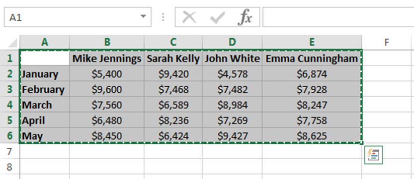
To transpose the data in Excel, first copy it by pressing the Ctrl+C shortcut keys.
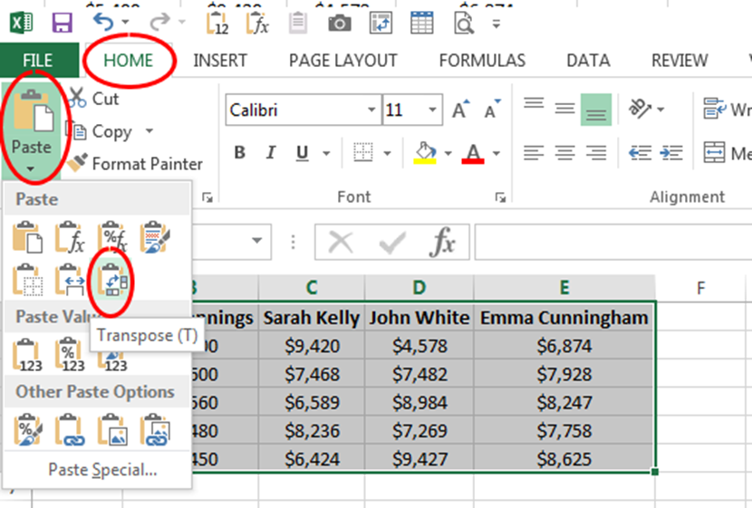
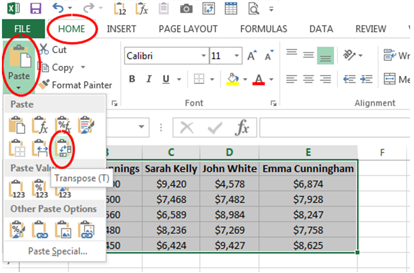
Click on the cell in the worksheet where you want to paste the transposed data and then click on the Home tab in the ribbon. In the Clipboard group click on the down arrow on the Paste command button to open a sub menu. Next you click on the Transpose button.

The data is now transposed. The sales people are therefore across the rows and the months are in columns. If you want, you can delete the original data if it is not needed.
Note: When you transpose data using the Paste Special Transpose button, the data is not dynamic. This means that when the original data source is changed, the transposed data stays the same because the data is just copied and pasted.
2. Excel Transpose Function
The Excel Transpose function is another way to transpose data in Excel. To flip the data with this function, you have to insert an Excel formula in the cells of the worksheet.

The Excel Transpose function contains just one argument which is the array argument. This is a required argument and is the range of cells that you want to transpose.
Let’s look at an example of how to flip data in Excel using the Excel Transpose function.
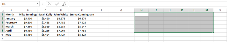
I will use the same data set as the one I used for the first method. The first thing to do is highlight the cell range where you want the data to be transposed to. Remember you want to transpose the rows to columns and vice versa. In this example, the data contains six rows so I highlight six columns. There are five columns in the data so I therefore highlight five rows. The cell range is therefore H1:M5.

In the top left cell of the selected range, in this example cell H1, I type the formula =TRANSPOSE(A1:E6). The range argument of the Transpose function is range A1:E6 in this example.

The Excel Transpose function is an array formula so you need to press Control + Shift + Enter on your keyboard after you have typed the formula in the cell. To see more examples of array formulas and how they work, then please see my post on how to find the first non blank cell in a row.
Note: When you Transpose data using the Excel Transpose function, the transposed data is dynamic. This means that when the original data source is changed, the transposed data will automatically update.
Paste Special Transpose vs the Excel Transpose Function
Which is the better method to transpose the data? The paste special Transpose method is definitely the easier and quickest to do. However, I prefer the Excel Transpose function because if the source data is changed then so does the transposed data. It is basically a dynamic transposed version of the source data.
Using Pivot Tables to Transpose Data in Excel
Another quick and easy way to transpose data is by using a pivot table. You can very easily move the pivot items from the rows section to the columns section and vice versa. To learn more about pivot tables, including how to create one, then please see my tutorial on how to make a pivot table in Excel. I have also written a whole book about pivot tables called Excel Bible for Beginners: The Step by Step Guide to Create Pivot Tables to Perform Excel Data Analysis and Data Crunching. You can purchase this book from my shop or click the Buy Now button below.

Excel Indirect Function
Another Excel function you can use that will transpose data in Excel is the Indirect function. Let’s look at a couple of examples on how to do this. The first example will show you how to transpose the data from columns to rows. The second example will show you how to transpose the data from rows to columns.
Transpose Data in Excel from Columns to Rows

In this example there are sales figures for each month. As you can see in the screenshot above, the months and sales are in columns A and B. I want to transpose the data so the months and sales are in rows.
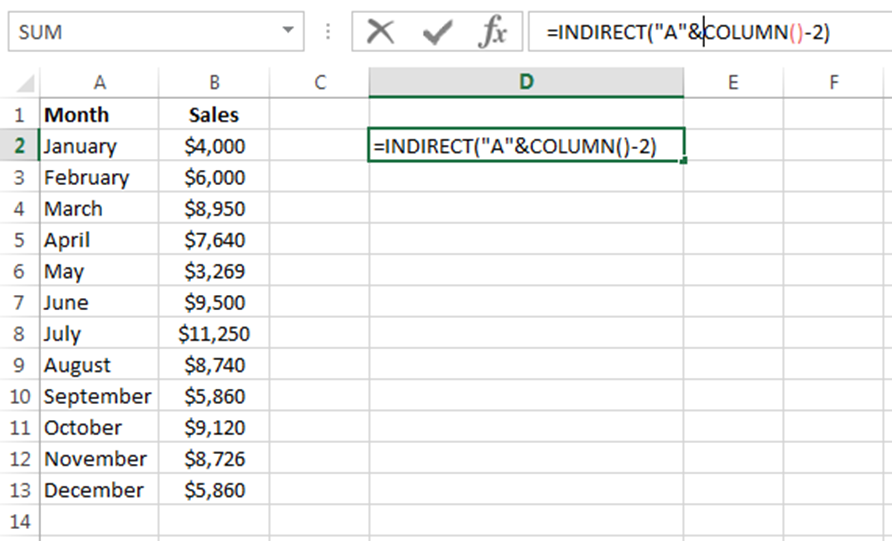
In cell D2, I enter the following formula =INDIRECT(“A”&COLUMN()-2).

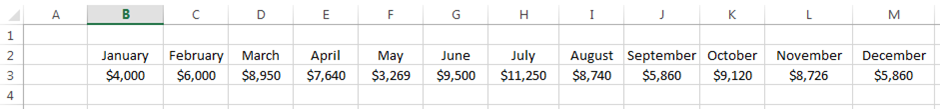
In cell D3, I enter the formula = INDIRECT(“A”&COLUMN()-2).

I then use the fill handles to copy the formulas across to column O. The months and sales figures are now across rows 2 and 3. To make the data neater, you can format the sales figures into the appropriate currency.
Transpose Data in Excel from Rows to Columns
In this example, the months and the sales figures are across the rows and I want to transpose them in columns. This method is different to the previous example. You cannot just replace the COLUMN function with the ROW function. Instead you have to include the ADDRESS function with the INDIRECT and ROW function.
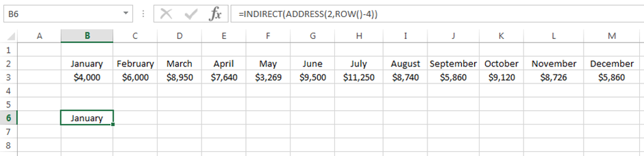
In cell B6 I enter the following formula =INDIRECT(ADDRESS(2,ROW()-4)).

In cell C6 I enter the formula =INDIRECT(ADDRESS(3,ROW()-4)).

I then just copied the formulas down to row 17 using the fill handles. The data has been transposed from rows to columns. To make the data neater, you can format the sales figures to the currency you require.
I hope you enjoyed this post on how to transpose data in excel. If you have any questions or feedback then please leave a comment below. I am very appreciative of your comments.
Learn More Excel Tips and Tricks
Transposing data in Excel is a great tip to use in Excel. If you want to learn more great tips, tricks and shortcuts in Excel to save you time and become more productive then you must buy my book Excel Bible for Beginners: Microsoft Excel Book Containing the Best Excel Tools, Tips and Shortcuts you Need to Know.
This Excel book will help you work smarter, save time, and become more productive by learning all the best hints, tips and tricks Excel has to offer. This book will show you how to:
- Hide specific text in a worksheet
- Quickly insert multiple rows using shortcut keys
- Shift between lots of open Excel windows
- Repeat your last actions using just one keystroke
- Get quick access to your favourite command buttons
- Use the Camera tool
- Quickly remove duplicate entries using the Advanced Filter tool
- Format dates from US to UK format and vice versa
- Make Excel speak back at you
- Automatically populate data
- Change data from column format to row format and vice versa
- Make your worksheets very hidden
- Analyse large datasets using Pivot Tables
- Create two-way lookups
- Access hidden features that are not available in the ribbon
- Use some Excel formulas and functions to manipulate data quickly
- And much more!
Here are just some reviews from Amazon for this book.


To learn more about this book or to purchase it from Amazon, then press either of the button below. You can also buy an eBook version in my shop.
More Excel Resources
Digital.com have released a comprehensive Excel resource which caters for all skill levels to improve their Excel skills. This resource covers Excel basics to advanced formulas and functions. To see the guide please click the link below:
