How to Remove First Four Characters in Excel

You may have a workbook which contains text but you only want to extract certain characters from it. For example, you may only want to extract the first name from a cell which contains both the first and last name of a person. In this tutorial, I will show you how to manipulate text and in particular, I will show you some great techniques of how to remove the first four characters in Excel using the following functions:

1) Excel RIGHT Function

2) Excel MID Function

3) Excel REPLACE Function

1. Using the RIGHT Function to Remove the First Four Characters in Excel

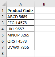
In this example, there is a list of product codes. I want to remove the first four characters and leave the last four numbers from the product code.

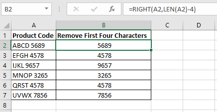
The formula =RIGHT(A2,LEN(A2)-4) in cell B2 is used to remove the first four characters in the product code. I have then copied the formula down to cell B7 using the fill handle.

How Does the Formula Work?

So how does this formula work? Let’s break this down so you can understand how it calculates. I will use the formula in cell B2 for the explanation.

Right Function

The Excel RIGHT function extracts a given number of characters from the right side of a specified text. For example =RIGHT(“Aeroplane”,4) will result in “lane”.

Len Function

The LEN function extracts the length of a given string. For example =LEN(“Aeroplane”) will result in 9 as there are 9 characters in the string “Aeroplane”.

RIGHT(A2,LEN(A2)

This section of the formula will return 9. In the first argument of the RIGHT function, you have to specify what text to use. In this example it is cell A2. For the second argument, you have to specify the number of characters you want to extract. For this argument, I am using the LEN function. This returns the number of characters of the product code ABCD 5689 which is 9. The space between ABCD and 5689 counts as a character. The formula =RIGHT(A2,LEN(A2) translates to =RIGHT(A2,9) which returns ABCD 5689.

RIGHT(A2,LEN(A2)-4)

I want to remove the first 4 characters so therefore I include a -4 at the end of the formula. LEN(A2)-4 therefore returns 5 (9-4=5). If I simplify this further, the RIGHT function is =RIGHT(A2,5) and returns 5689.

How to Remove the First nth Character of a String

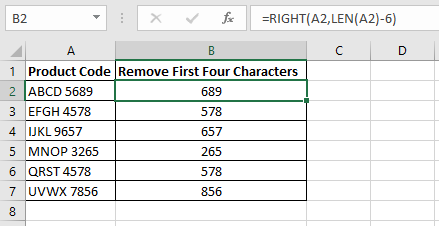
If you want to remove the first nth characters in a string you just change the -4 to whatever number of characters you want to remove. For example, if you want to remove the first six characters of a string then simply change the -4 to -6. If you want to remove the first two characters then change it to -2 and so on.

2. Using the Excel MID Function to Remove the First Four Characters in Excel

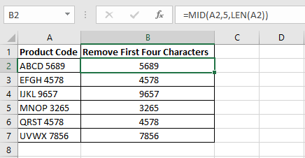
You can also perform the same feat of removing the first four characters of a string using the Excel MID function. The formula in cell B2 is =MID(A2,5,LEN(A2)). I then just copied the formula down using the fill handle.

How Does the Formula Work?

MID Function

The Excel MID function extracts the middle of a text based on the specified number of characters. For example, =MID(“Aeroplane”,3,4) returns “ropl”. The first argument is the text string or a cell reference you want to extract from. The second argument is the location number you want to start the extraction from. The third argument is the number of characters you want to extract.

MID(A2,5

This section of the formula says to start from the fifth character of the product code ABCD 5689. This means that it will start the extraction from the space after ABCD. This is because the space is the fifth character along from the left.

LEN(A2)

The LEN function is returning the number of characters of the product code ABCD 5689 which is 9.

MID(A2,5,LEN(A2))

If you simplify this formula, the MID function is =MID(A2,5,9). It starts from the space and extracts 9 characters along. Because there is only 4 characters after the space it therefore extracts 5689.

How to Remove the First nth Character of a String

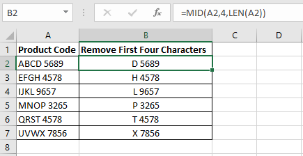
If you want to remove the first nth character then just add a 1 in the MID functions second argument. For example, if I want to remove the first three characters, I enter 4 in the MID functions second argument as shown in the above screenshot. Here you can see that ABC has been removed. If I want to remove the first two characters, I just enter 3 for the second argument.

3. Using the Excel Replace Function to Remove the First Four Characters in Excel

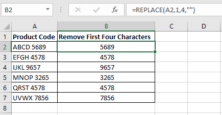
Another way you can remove the first four characters of a text string is by using the Excel REPLACE function. The formula in cell B2 is =REPLACE(A2,1,4,””). I then copied the formula down using the fill handle.

How Does the Formula Work?

REPLACE Function

The Excel REPLACE function replaces a set of characters in a string with another set of characters. The first argument of the REPLACE function is the string or the cell you want to replace the characters with. The second argument is the position of the old text to begin replacing characters. The third argument is the number of characters you want to replace the old text with. The fourth argument is the new characters you want to replace the old text with.

REPLACE(A2,1,4,””)

The first argument is the product code in cell A2. The second argument is the start number. I want to start from the beginning so I enter a 1. The third argument is 4 as I want to replace the first four characters with new text. The last argument is two quotation marks which means a blank string. I want to replace the first four characters with a blank string so I am left with the last 4 characters.

How to Remove the First nth Character of a String

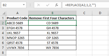
To remove the first nth character, just replace the third argument with the number of characters you want to remove. For example, if you want to remove the first two characters then just change the third argument to 2 as shown in the screenshot above.

I hope you enjoyed this tutorial on how to remove the first four characters in Excel. If you have any questions or feedback then please leave a comment below.

Gifts for Spreadsheet Gurus: Excel Mugs to Fuel Your Productivity!

Ready to take your Excel experience to the next level? Our exclusive Excel mugs are the perfect blend of functionality and style. Whether you’re a spreadsheet enthusiast, an Excel guru, or you simply want to add a touch of data-driven flair to your workspace, these spreadsheet mugs have you covered. Don’t miss out on the opportunity to sip, savor, and spreadsheet in style. Click now to browse our collection and choose your new favorite Excel mug!

Learn to Create More Powerful Excel Formulas

If you want to create even more powerful formulas then you can purchase my Excel book called Excel Formulas and Functions: The Step by Step Excel Guide on how to Create Powerful Formulas. This book will teach you how to create formulas using advanced Excel functions such as SUMPRODUCT, SUBSTITUTE, REPT, SEARCH, FIND and many more. You will learn how to create Excel array formulas and what array constants are. After reading this book, you will be able to perform magic with Excel formulas.

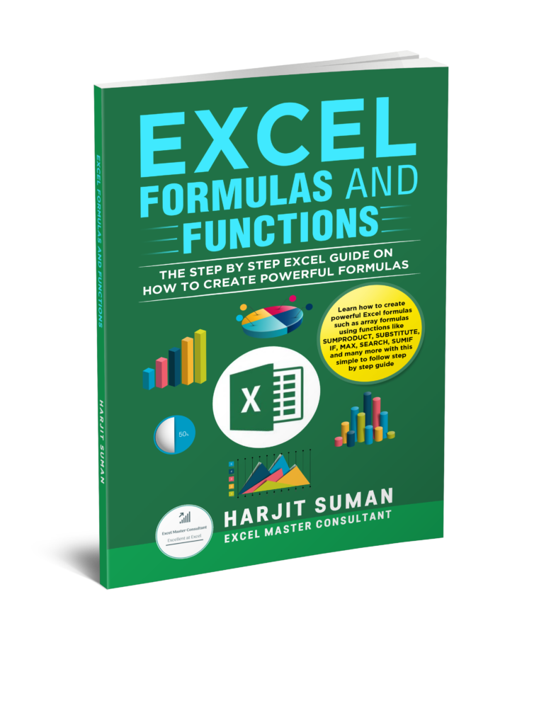
Here are some reviews from people who have purchased this book.

To learn more about this book and to purchase it from Amazon, then simply click one of the buttons below.