This tutorial will teach you how to do VLOOKUP in Excel. The Excel VLOOKUP function is one of the most popular and useful functions available. If you find that you are continually extracting data from various tables then consider learning the VLOOKUP function. Once you have learned how to use VLOOKUP in Excel from this tutorial, you will save valuable time and effort going forward. In this tutorial, I will explain what the VLOOKUP function is and how to do VLOOKUP in Excel.
What is the Excel VLOOKUP Function?
The VLOOKUP function allows you to extract a value from a given column in a table by looking at the lookup value. The lookup value must appear in the first column of the table. The values you want to extract must appear in the columns to the right. VLOOKUP stands for vertical lookup because you are searching for a value in a column. You can think of VLOOKUP as a phonebook. You are searching for the name of a person you know on the left to extract their phone number to the right of the persons name.
Syntax
The syntax for the VLOOKUP function is:
=VLOOKUP(lookup_value, table_array, col_index_num, [range_lookup])
Arguments
lookup_value – The value you are looking for in the left most column of the table
table_array – The table from which you want to retrieve the value
col_index_num – The column number in the table_array in which you want to retrieve the value
[range_lookup] –This is optional. If you select FALSE or a 0 then it is an exact match. If you select TRUE or a 1 then it is an approximate match
Now let’s have a look at an example of how to use VLOOKUP to extract an exact match and then an approximate match.
How to do VLOOKUP in Excel to Extract an Exact Match
Using VLOOKUP to extract an exact match is the most common method of using the VLOOKUP function.

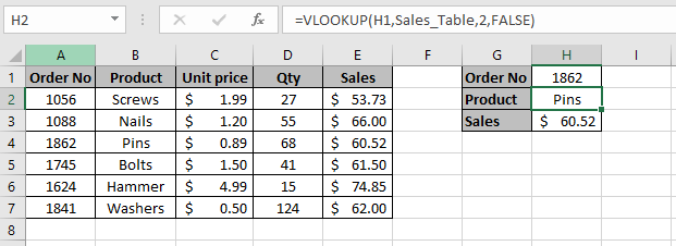
In this example, there is a sales table for a hardware store in the range A1:E7 which shows the total sales in column E for each product in column B. This sales table will be the lookup table. In cell H2, I want to extract the product and in cell H3, I want to extract the total sales for the order number in cell H1. The lookup value is the order number in cell H1 which I will use to extract the information I need.
The first thing I need to do is enter the VLOOKUP formula in cell H2 to extract the product. Here are the steps to do this:

1. Click in the cell where you want to enter the VLOOKUP formula. In this example it will be cell H2
2. Click on the Insert Function box which is to the left of the Formula Bar. The Insert Function dialog box will appear
3. In the Search for a function field type VLOOKUP and then press the Go button
4. Under Select a function select VLOOKUP and then press the OK button

5. The Function Arguments dialog box will appear. The first thing to do is enter the lookup value. The lookup value in this example is the order number in cell H1 so I select cell H1 in the Lookup_value field
6. The next thing to do is enter the range where the lookup table is. The lookup table is the table in the range A1:E7 so I select this range in the Table_array field
7. I now need to enter the column number where the Product column is in the lookup table. The products are listed in the second column of the lookup table so I enter 2 in the Col_index_num field
8. Lastly, I want to do an exact match. For an exact match, you enter a FALSE or a 0 in the Range_lookup field
9. Once all the fields are entered, press the OK button

The VLOOKUP formula returns “Pins”.
Note: The lookup value column, i.e. the order number column, must be in the left most column of the lookup table. This is because the VLOOKUP only searches to the right.

To extract the sales for the order number in cell H1, you just follow steps 1 to 9 again. The only difference is that I want to extract the sales this time which is in the fifth column of the lookup table, so I enter 5 in the Col_index_num argument.
How to do VLOOKUP in Excel to Extract an Approximate Match
In some instances, you may have a set of data where you cannot extract an exact match from a lookup value. In this case you will need to extract the best match for the lookup value.

In this example, there is a list of Sales people with their sales in column C. I want to enter the commission % each Sales people will earn in column D based on their sales in column C. To help me with this, there is a lookup table in the range G1:H7. This lookup table shows how much commission a Sales person will earn in column H based on the sales achieved in column G. The reason why we need to do an approximate match is because the sales in column C, which is the lookup value does not match the sales in the lookup table in column G. If I did an exact match by entering a FALSE in the VLOOKUP’s fourth argument, it will return #N/A.
The first thing to do is to enter the VLOOKUP formula in cell D2 to find out how much commission Peter has achieved. To do this follow these steps:

First select cell D2 and then follow steps 1 to 4 as per the previous example until the Function Arguments dialog box appears. Next you need to fill in all the arguments.
Lookup_value – The lookup value is the sales amount in cell C2 so I select cell C2
Table_array – This is the lookup table in the range G1:H7. Notice that I have made this range absolute by putting dollar signs ($) before and after the column and row references. This is because I will be copying the VLOOKUP formula down column D and if I didn’t make this range absolute, it will give incorrect results.
Col_index_num – I am extracting the commission % in column H which is the second column in the lookup table so I enter 2
Range_lookup – I want to do an approximate match so I enter TRUE. I could also enter a 1 instead
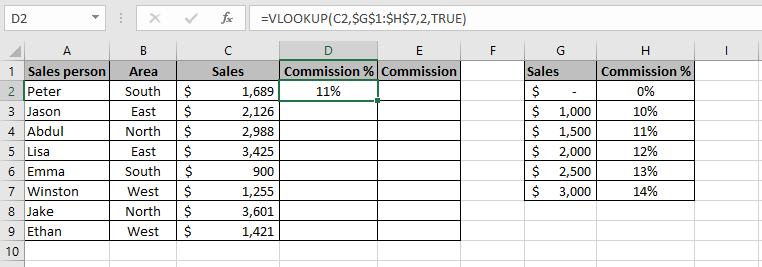
Once I press the OK button the VLOOKUP function returns 11% in cell D2.

You can then copy the formula down column D using the Fill Handle to get the commission for all the Sales people as shown in the screenshot above.
Notice how the VLOOKUP approximate match works. If the VLOOKUP function cannot find the exact sales value in column G, it will return the next smallest value. Let’s now look at some of the results in column D to understand how the VLOOKUP approximate match is calculated.
In cell D2, the commission rate is 11% as the sales of $1,689 is above $1,500 but below $2,000 so it uses the smallest value of the two which is $1,500. The commission for $1,500 is 11%.
In cell D3, the commission rate is 12% as the sales of $2,126 is above $2,000 but below $2,500 so it uses the smallest value of the two which is $2,000. The commission for $2,000 is 12%.
In cell D4, the commission rate is 13% as the sales of $2,988 is above $2,500 but below $3,000 so it uses the smallest value of the two which is $2,500. The commission for $2,500 is 13%.
In cell D5, the commission rate is 14% as the sales of $3,425 is above $3,000. Anything above $3,000 will earn a commission of 14%.
In cell D6, the commission rate is 0% as the sales of $900 is below $1,000. Anything below $1,000 will earn a commission of 0%.
Useful Tip
It is very good practice to name your lookup table. This is particularly true if you have a lot of VLOOKUP formulas in your spreadsheet. By doing this, you will know which tables the VLOOKUP formulas are referring to if you have given them relevant names and is much easier to understand than looking at cell references in your formula.

To name your lookup table simply select the table and then name it in the Name Box and then press Enter on your keyboard. If you are using more than one word to name the table then you can’t have a space between the words. You should name it so that it is relevant to what the table is showing. In this example, I have called the table “Sales_Table”. I could have also named it “SalesTable”.

The VLOOKUP formula in cell H2 is =VLOOKUP(H1,Sales_Table,2,FALSE) and in cell H3 the formula is =VLOOKUP(H1,Sales_Table,5,FALSE). This is far easier to understand than having the third argument in the VLOOKUP formula as a cell reference.
How to use VLOOKUP in Excel Video
If you want to learn more about how to use VLOOKUP in Excel, then please see my video below which contains further examples of how to do VLOOKUP in Excel and how to use it to extract an exact and approximate match.
Limitations of VLOOKUP
The VLOOKUP function is a great tool to extract information from tables and is one of the most popular Excel functions available. Although it has great benefits, it also comes with some limitations. You can see my post on the limitations of VLOOKUP to learn more about this.
Learn More About Excel Formulas and Functions
If you want to learn more about VLOOKUP or any other lookup functions such as HLOOKUP, INDEX+MATCH then I have written a book on Excel formulas and functions. As well as lookup functions, this Excel book will teach you other functions too such as logical, text, summing and counting functions. You can purchase my comprehensive Excel formulas and functions book from Amazon. The book is called Excel Formulas and Functions: The Complete Excel Guide For Beginners.

Here are some of the reviews from people who have purchased this book:


To learn more about this book and to purchase it from Amazon, then simply click one of the buttons below.
I hope you enjoyed my post on how to do VLOOKUP in Excel. I would really appreciate your feedback and comments on this tutorial. If you have any feedback or questions then please leave a message in the comments section below. I am always grateful to hear from my readers.

Great post. I have followed the examples in this post and I am a lot more confident in using VLOOKUP now. Thank you!
Hi Gemma,
Thank you for your comment. I am glad you found this post helpful. If you need any more help then please let me know.