Combine Two Cells in Excel: In 3 Simple Ways

There are various methods you can use to combine two cells in Excel. A common reason to merge cells is to format a heading. Another reason to combine two cells in Excel is if a persons first and last name are in separate cells. You may want both names in one cell. In this Excel tutorial, I will show you the best ways to merge cells in Excel. You will learn how to merge cells by using the:

1. Excel CONCATENATE function
2. Ampersand (&) symbol
3. Merge & Center button

1. How to Combine Two Cells in Excel using the CONCATENATE Function

In the screenshot above, there is a list of first and last names in columns A and B. The goal is to merge the two names in one cell in column C. To do this, we can use the Excel CONCATENATE function. Concatenate means “to join” or “to combine”. The CONCATENTATE function combines text from different cells into one cell. Now lets see how we do this.

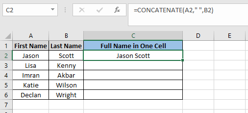
In cell C2, I want to combine cells A2 and B2 together. I have therefore used these cells as the arguments in the CONCATENATE function. The formula is:

=CONCATENATE(A2,” “,B2)

Notice I have double quotation marks (” “) in the second argument. This means there is a space between the first and last name. If you don’t want a space between the two cells then just take out the double quotation marks (” “). The formula will therefore be:

=CONCATENATE(A2,B2)

You can then use the fill handle to copy the formula down.

2. How to Combine Two Cells in Excel using the Ampersand Symbol

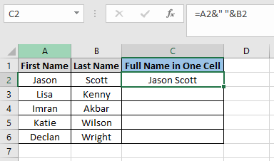
You can also use the ampersand (&) symbol to merge cells in Excel. This is very similar to the first method where we use the CONCATENTATE function. You use the ampersand symbol before every text you want to join. The formula in cell C2 is:

=A2&” “&B2

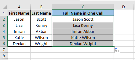
You can then copy the formula down using the fill handle.

Notice again I used double quotation marks (” “) after the first ampersand symbol. This is so that I have a space between the first and last name. If you don’t want a space then the formula will be:

=A2&B2

3. Use the Merge & Center Button to Merge Cells in Excel

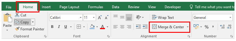
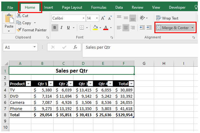
You can also use the Merge & Center command button to combine cells in Excel. This button is located in the Excel ribbon under the Home tab in the Alignment group.

Using the Merge & Center button is best used for formatting your worksheet. This is particularly useful for table headings or if there is a large heading in your worksheet and you want it to look neater. Now lets have a look at an example of how to use the Merge & Center command button to merge cells in Excel.

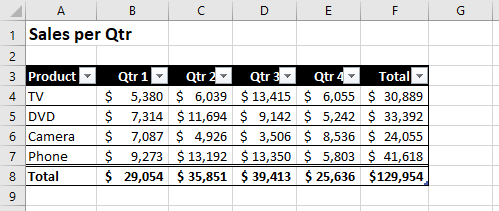
In the example above, there is a data table showing sales per quarter for some electrical items. Notice the title in cell A1. We can format this better by having the title go across the length of the table in cells A1:F1.

Here are the steps to do this.

1. Select the range where you want to merge and centre the title. In this example, I want to have the title go across the range A1:F1 so I select this range

2. Select the Home tab and then under the Alignment group click on the Merge & Center command button

The Merge & Center button combines the selected cells into one cell and centres the text.

The Problem with the Merge & Center Button

The Merge & Center buttons is a great way to combine cells in Excel but it does have one major flaw. It combines two or more cells together but not the text within the cells. Lets look at an example using the dataset with the first and last names.

As you can see in the above example, the first name in cell A2 is preserved. The last name in cell B2 is removed. Using the Excel CONCATENATE or ampersand symbol is the best method for combining two or more cells in Excel for this particular exercise.

Excel does give you a warning whenever you press the Merge & Center button. If you press OK then it will go ahead and merge the cells together.

Advanced Techniques on How to Merge Cells

More than likely you may need to do more than combine two cells in Excel. This section will show you a couple of advanced techniques in how to combine cells in Excel.

How to Write a Sentence within Combined Cells in Excel

You may want to write a sentence by merging two or more cells.

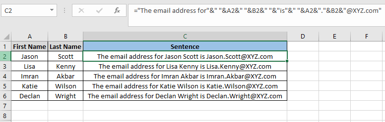
Lets use the same dataset we used for the first two methods which contains the first and last names in columns A and B. We can write a sentence in cell C2 which says “The email address for Jason Scott is Jason.Scott@XYZ.com“. To do this the formula in cell C2 will be:

=”The email address for”&” “&A2&” “&B2&” “&”is”&” “&A2&”.”&B2&”@XYZ.com”

Notice you can write a text string in the formula itself. A text string doesn’t have to be written in a cell and then that cell be combined in the formula. The text string must have quotation marks (“) before and after the string. It must also be followed by an ampersand symbol. You must also remember to include any spaces and be placed in the correct location. Once you are happy with the formula you can then copy it down the column.

How to Display Formatting within Combined Cells in Excel

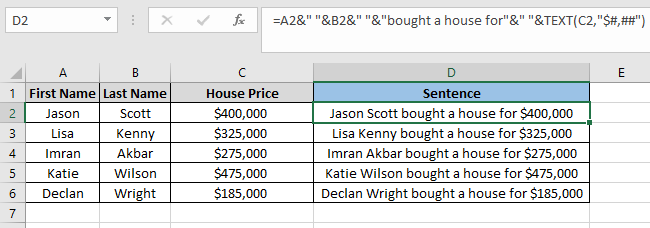
If the cells you want to combine contains formatting such as currency then the formula will not contain the formatting. For example, in the data above we have the same list of names in columns A and B. Column C contains the price they bought their house. In cell D2, I want to combine cells A2, B2 and C2 to read “Jason Scott bought a house for $400,000”. If I used the formula:

=A2&” “&B2&” “&”bought a house for”&” “&C2

The result will be “Jason Scott bought a house for 400000”. I would like to include the currency and a comma separator after the hundred thousand number. In order to do this we have to use the TEXT function. The revised formula will be:

=A2&” “&B2&” “&”bought a house for”&” “&TEXT(C2,”$#,##”)

The TEXT function contains two arguments. The first argument is value. This is the cell you want to format. In this instance it is cell C2. The second argument is format_text. This is how you want to format the text. To display the USD symbol I enter “$”. I then use “#,##” to display the house price with a comma separator after the first hashtag. If I wanted to show two decimal places I would enter “$#,##.00”. You can then copy the formula down the column.

Additional Information

If you would like to learn about the Excel TEXT function then please click here.

For more Excel tutorials then please visit my Excel Tutorials page. You will find lots of tutorials to help you improve your Excel skills. Please also take the time to visit my shop. In here, you will find lots of books on a variety of topics to take your Excel skills to the next level.

I hope you enjoyed this Excel tutorial on how to combine two cells in Excel. If you have any questions or feedback please leave them in the comments section below.

Excel in Style: Shop the Best Collection of Excel Mugs Now!

Unlock productivity with every sip! Our Excel mugs are the perfect blend of style and function, designed to fuel your data-driven journey. Whether you’re a spreadsheet whiz or just appreciate a quality mug, these are your secret weapon. Don’t wait – click below to explore our exclusive collection and make every coffee break a spreadsheet sensation!